Implementing a Custom Logistic Regression Estimator in Scikit-Learn with JAX
Scikit-learn has become an indispensable tool for data analysis and modeling in Python. While it offers a wide array of built-in estimators, there are scenarios where implementing a custom algorithm becomes necessary, either to meet specific requirements or to experiment with novel approaches. Fortunately, scikit-learn provides a flexible framework for creating custom estimators that seamlessly integrate with its ecosystem. In this blog post, we'll explore how to implement a custom Logistic Regression estimator using JAX for optimization, leveraging scikit-learn's utilities for cross-validation, hyperparameter tuning, and metric reporting.
Introduction to JAX
Before we dive into the implementation, let's briefly introduce JAX. JAX is a NumPy-like framework for numerical transformations that utilizes hardware optimizations from TensorFlow's XLA (Accelerated Linear Algebra) at the CPU or GPU level. This allows JAX to be considerably faster and more efficient than traditional NumPy operations, making it an excellent choice for implementing custom machine learning algorithms.
Logistic Regression: Theory and Algorithm
Let's review the theory behind logistic regression and derive the key equations.
Logistic regression is a classification algorithm that estimates the probability of an instance belonging to a particular class. The core of logistic regression is the sigmoid function:
$$ \sigma(z) = \frac{1}{1 + e^{-z}} $$where the signal $z$ is a linear combination of the input features $x$ and weights $w$, plus a bias term $b$:
$$ z = w^T x + b $$JAX allows us to use `jnp.exp` to specify exponents:
def sigmoid(self, X):
    return 1 / (1 + jnp.exp(-X))

#and
h = self.sigmoid(jnp.dot(X, param) + bias)
For a given input vector $x$, the probability of belonging to the positive class is modeled as:
$$ P(y=1|x) = \sigma(w^T x + b) $$where $w$ is the weight vector and $b$ is the bias term.
The error measure should capture how well our model predicts the output class given a set of input features. Assuming that the data points are independent and identically distributed, the likelihood of observing the entire dataset is the product of the individual probabilities:
$$ L(w) = \prod_{n=1}^{N} P(y_n|x_n) = \prod_{n=1}^{N} h(x_n)^{y_n} (1 - h(x_n))^{(1-y_n)} $$To simplify calculations and avoid numerical underflow, we often work with the log-likelihood:
$$ \log L(w) = \sum_{n=1}^{N} [y_n \log h(x_n) + (1-y_n) \log(1 - h(x_n))] $$Maximizing the log-likelihood is equivalent to minimizing the negative log-likelihood:
$$ -\log L(w) = -\sum_{n=1}^{N} [y_n \log h(x_n) + (1-y_n) \log(1 - h(x_n))] $$Dividing the negative log-likelihood by the number of data points $N$ gives us the average cross-entropy loss:
$$ E_{in}(w) = \frac{1}{N} \sum_{n=1}^{N} [-y_n \log h(x_n) - (1-y_n) \log(1 - h(x_n))] $$This is precisely the binary cross-entropy loss function, which quantifies the difference between the predicted probabilities and the true labels. To prevent overfitting, we can add a penalty term to the loss function that discourages large weights. A common choice is the L2 regularization term: $\frac{\lambda}{2} ||w||^2$, where $\lambda$ is the regularization strength.
Adding the L2 regularization term to the cross-entropy loss gives us the final loss function used in logistic regression with L2 regularization:
$$ E_{in}(w) = \frac{1}{N} \sum_{n=1}^{N} [-y_n \log h(x_n) - (1-y_n) \log(1 - h(x_n))] + \frac{\lambda}{2} ||w||^2 $$where $N$ is the number of data points, $x_n$ is the input feature vector for the $n$-th data point, $y_n$ is the corresponding true label (0 or 1), and $w$ and $b$ are the weights and bias, respectively.
We implement the above as the loss function in our class:
def _loss(self, param, bias, X, y):
    h = self.sigmoid(jnp.dot(X, param) + bias)
    N = y.size
    h = jnp.clip(h, 1e-14, 1 - 1e-14)
    base_loss = -jnp.sum(y * jnp.log(h) + (1 - y) * jnp.log(1 - h))/N
    reg_loss = 0.5 * self.lmbd * (jnp.dot(param, param) + bias**2)
    return base_loss + reg_loss
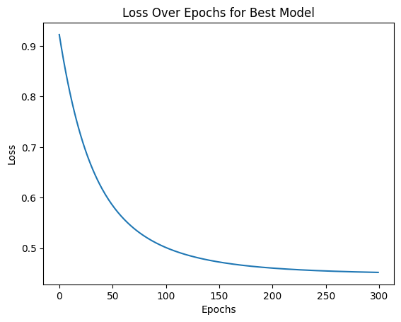
The loss function for logistic regression with L2 regularization is not easily minimized analytically by setting its gradient to zero. Therefore, we resort to an iterative optimization technique called gradient descent. Gradient descent starts with an initial guess for the weights and iteratively updates them in the direction of the negative gradient of the loss function. This process gradually reduces the loss and eventually converges to a local minimum. The update rule for gradient descent is given by:
$$ w_{t+1} = w_{t} - \eta \Delta E_{in}(w_{t}) $$where $w_{t}$ is the weight vector at iteration $t$, $\eta$ is the learning rate, and $\nabla E_{in}(w_{t})$ is the gradient of the loss function with respect to $w$ at iteration $t$.
Algorithm: Logistic Regression with Gradient Descent
- Initialize $w_{(0)}$ (e.g., to zeros or small random values).
- For $t = 0, 1, 2, \dots$:
- Compute the gradient: $g_t = -\frac{1}{N} \sum_{n=1}^N \frac{y_n x_n}{1 + e^{y_n w_{t}^{T}x_n}} + \lambda w{t}$
- Set the direction to move: $v_t = -g_t$
- Update the weights: $w_{t+1} = w_{t} + \eta v_t$
- Iterate to the next step until a stopping criterion is met (e.g., based on a maximum number of iterations, or until the change in loss is small enough).
- Return the final weights $w$.
This algorithm iteratively updates the weights using the gradient of the logistic regression loss function until a stopping criterion is met. In our implementation, we use a basic stopping criterion based on a tolerance limit. The learning rate $\eta$ controls the step size of the updates and needs to be carefully chosen to ensure convergence.
We now implement the fit function based on gradient descent:
def fit(self, X, y):
    check_X_y(X, y); X = jnp.array(X); y = jnp.array(y)
    self.param = 1.0e-5 * jnp.ones(X.shape[1])
    self.bias = 1.0
    loss = float(self._loss(self.param, self.bias, X, y))
    for epoch in range(self.epochs):
        self.param -= self.lr*grad(self._loss, argnums=0)(self.param, self.bias, X, y)
        self.bias -= self.lr*grad(self._loss, argnums=1)(self.param, self.bias, X, y)
        loss = self._loss(self.param, self.bias, X, y)
        self.losses.append(loss)
        if epoch > 20:
            if jnp.abs(self.losses[-1] - self.losses[-20]) < self.tolerance:
                print(f'Early stopping at epoch {epoch}')
                break
    self._is_fitted_ = True
    return self
Implementing the Custom Logistic Regression Estimator
We'll create a `LogisticClassifier` class that inherits from scikit-learn's `BaseEstimator` and `ClassifierMixin`. This allows our custom estimator to work seamlessly with scikit-learn's utilities.
Let's break down the implementation and explain each part:
import jax.numpy as jnp
from jax import grad
from sklearn.base import BaseEstimator, ClassifierMixin
from sklearn.utils.validation import check_X_y

class LogisticClassifier(BaseEstimator, ClassifierMixin):
    def __init__(self, lr=0.01, epochs=1000, lmbd=0.01, tolerance=1e-5):
        self.param = None      # weights
        self.bias = None       # bias
        self.lr = lr           # learning rate
        self.epochs = epochs   # number of epochs
        self.losses = []       # list of losses
        self.lmbd = lmbd       # regularization parameter
        self.tolerance = tolerance  # convergence tolerance

    def get_params(self, deep=True):
        return {'lr': self.lr, 'epochs': self.epochs, 'lmbd': self.lmbd}

    def set_params(self, **params):
        if 'lr' in params:
            self.lr = params['lr']
        if 'epochs' in params:
            self.epochs = params['epochs']
        if 'lmbd' in params:
            self.lmbd = params['lmbd']
        return self
The `get_params` and `set_params` methods are required for compatibility with scikit-learn's model selection tools. They allow hyperparameter tuning using techniques like `GridSearchCV`.
    def sigmoid(self, X):
        return 1 / (1 + jnp.exp(-X))

    def _loss(self, param, bias, X, y):
        # same as before

    def fit(self, X, y):
        # same as before

    def predict(self, X):
        X = jnp.array(X)
        return self.sigmoid(X @ self.param + self.bias) >= 0.5
Using the Custom Estimator
Now that we have implemented our custom logistic regression estimator, we can use it just like any other scikit-learn estimator. Here's an example using the Titanic dataset:
import pandas as pd
from sklearn.model_selection import train_test_split
from sklearn.metrics import classification_report

df = pd.read_csv('/kaggle/input/titanic/train.csv')

X = df.drop(columns=['Survived', 'PassengerId'])
y = df['Survived']

X_train, X_test, y_train, y_test = train_test_split(X, y, test_size=0.1, random_state=42)

# Transforming features
X_train = pipeline.fit_transform(X_train, y_train)

param_grid = {
    'lr': [5e-3, 5e-2, 5e-1],
    'epochs': [300, 400, 500]
}
model = LogisticClassifier()
grid_search = GridSearchCV(model, param_grid, cv=5, scoring='accuracy', error_score='raise', n_jobs=-1)
grid_search.fit(X_train, y_train)
print(grid_search.best_params_)

# Print the classification report
print(classification_report(y_test, y_pred))
This custom implementation achieves comparable performance to scikit-learn's built-in logistic regression:
             precision    recall  f1-score   support

           0       0.88      0.78      0.82        54
           1       0.71      0.83      0.77        36

    accuracy                           0.80        90
   macro avg       0.79      0.81      0.80        90
weighted avg       0.81      0.80      0.80        90
Conclusion
In this blog post, we've explored how to create a custom logistic regression estimator using scikit-learn's base classes and JAX for optimization. This approach allows us to leverage the power of automatic differentiation and JIT compilation while still benefiting from scikit-learn's ecosystem of tools for model selection, evaluation, and preprocessing.
Custom estimators open up a world of possibilities for implementing novel algorithms, optimizing performance, and experimenting with different techniques. By following the scikit-learn API, we ensure that our custom estimators can seamlessly integrate with existing workflows and take advantage of the rich ecosystem of tools and utilities that scikit-learn provides.
Whether you're implementing a cutting-edge algorithm or fine-tuning an existing one for your specific use case, custom estimators in scikit-learn provide the flexibility and power you need to push the boundaries of your machine learning projects.